To find out more about OPeNDAP consult:
https://www.opendap.org/
! *********************************************************
! DEMO: Using Ferret and OPENDAP to access remote data sets
! *********************************************************
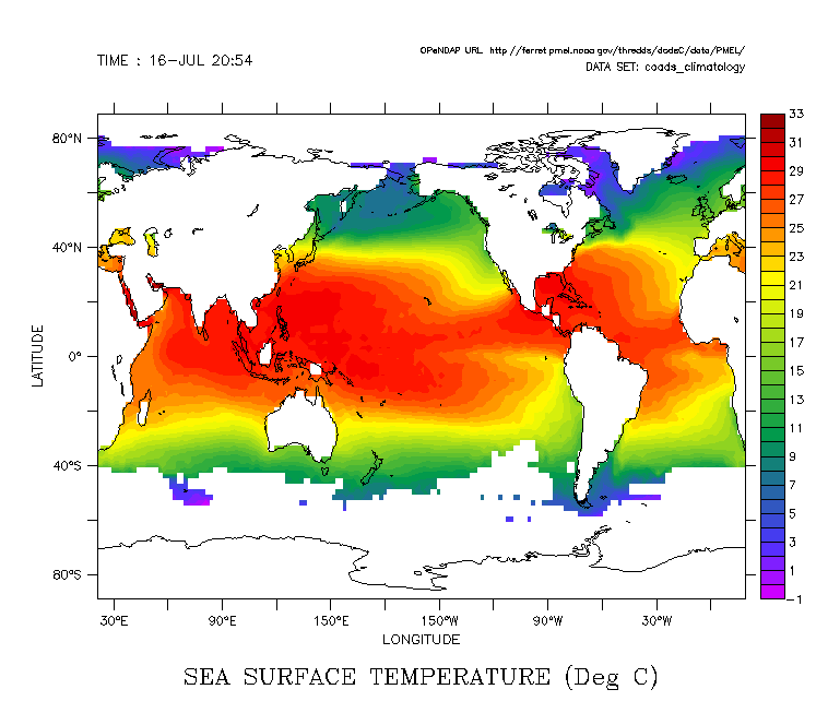
! First we will examine the COADS climatology dataset from the Pacific
! Marine Environmental Laboratory in Seattle, Washington.
! Note: Once the dataset has been initialized from the remote site,
! using the dataset is exactly the same as if it were local
currently SET data sets:
1> http://data.pmel.noaa.gov/thredds/dodsC/data/PMEL/coads_climatology.nc (default)
name title I J K L M N
SST SEA SURFACE TEMPERATURE 1:180 1:90 ... 1:12 ... ...
AIRT AIR TEMPERATURE 1:180 1:90 ... 1:12 ... ...
SPEH SPECIFIC HUMIDITY 1:180 1:90 ... 1:12 ... ...
WSPD WIND SPEED 1:180 1:90 ... 1:12 ... ...
UWND ZONAL WIND 1:180 1:90 ... 1:12 ... ...
VWND MERIDIONAL WIND 1:180 1:90 ... 1:12 ... ...
SLP SEA LEVEL PRESSURE 1:180 1:90 ... 1:12 ... ...
! SHOW DATA verifies that this is indeed a remote dataset
!
! Now let's look at a color contour of Sea Surface Temperature
yes? fill/t="16-jul" sst
yes? go land
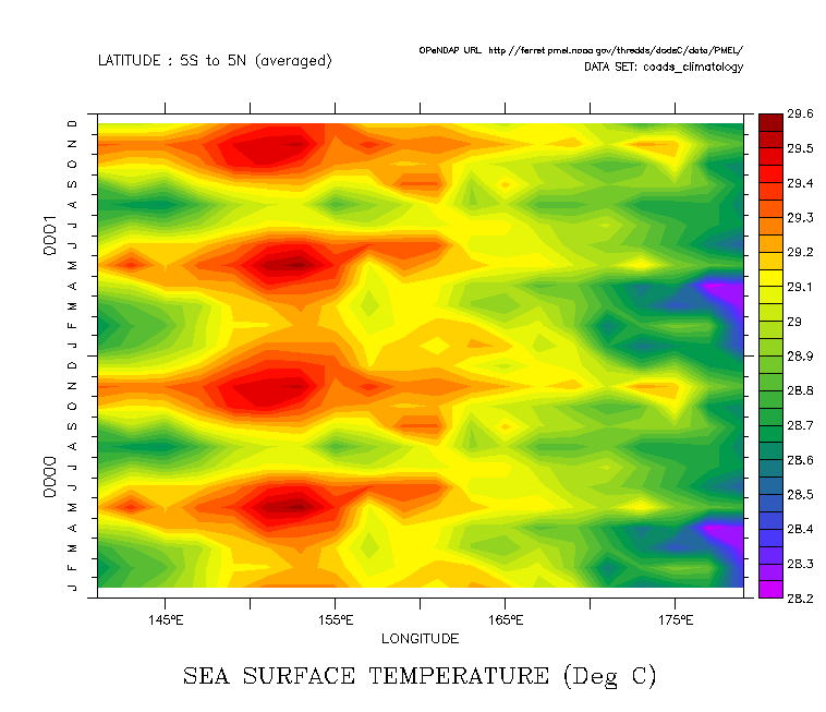
! Remote data has full random access. Here we will plot the evolution of SST
! averaged over the Equatorial waveguide (an XT section)
yes? fill/x=140E:180E/L=1:24 sst[Y=5S:5N@AVE]
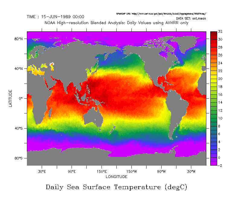
! Now, let's use a different SST dataset from the Earth System Research Laboratory
! (ESRL) in Boulder, Colorado
yes? use "http://www.esrl.noaa.gov/psd/thredds/dodsC/Aggregations/OISSThires/sst.mean.nc"
yes? show data 2
currently SET data sets:
2> http://www.esrl.noaa.gov/psd/thredds/dodsC/Aggregations/OISSThires/sst.mean.nc  (default)
name     title                             I         J         K         L         M         N
SST      Daily Sea Surface Temperature    1:1440    1:720     ...       1:12575   ...       ...
! This data set contains weekly mean global SST grids prepared by
! Reynolds et. al.
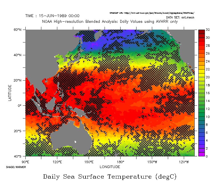
! Let's look at the SST for June 15, 1989
! Note this is a higher-resolution data which may take longer to load
yes? fill/t="15-JUN-1989" sst[d=2]
yes? go fland
! Plot a subset of the same timestep data. A faster response may be noticed due to Ferret data caching.
yes? fill/x=90e:110w/y=-40:60/t="15-JUN-1989" sst[d=2]
yes? go fland
! Now, let's see where the June 15, 1998 Reynolds field (served from Boulder)
! exceeds the June climatological data (served from Seattle)
! This requires regridding the 2x2 degree COADS data to the 0.25x0.25 degree
! Reynolds grid
yes? let coads_on_reynolds = sst[d=1,g=sst[d=2]]
yes? let warmer = IF sst[d=2] GT coads_on_reynolds THEN 1

yes? shade/over/pal=black/levels/pattern=weave/t="15-jun-1989" warmer
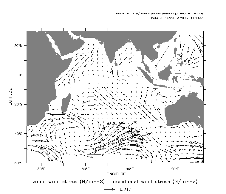
! Next let's look at a dataset from NASA's Earth Observing system (EOS) HDF-EOS group.
! This data set is in HDF format. It contains surface data - wind stress, heat flux,
! humidity, precipitable water.
yes? use "http://measures.gsfc.nasa.gov/opendap/GSSTF/GSSTF.3/2008/GSSTF.3.2008.01.01.he5"
! Note that OPENDAP gives Ferret format-independence -- the ability to read an HDF file
! Let's look at the wind-stress vectors in the Indian Ocean
yes? vector/x=20:140/y=-60:30 STU, STV
yes? go fland
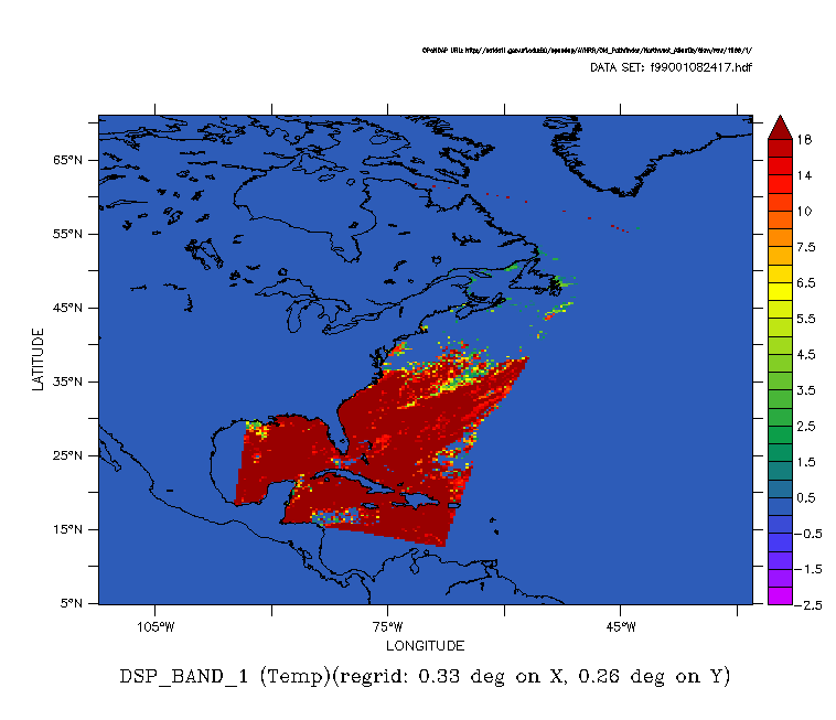
! Next lets examine some NOAA AVHRR data served by the University
! of Rhode Island, Graduate School of Oceanography (GSO). This
! data is in the form of 1024x1024 pixel images (1 megabyte per image)
! We will use this to illustrate the ability of Ferret and OPENDAP to
! subsample -- making the data transfer much faster.
yes? use "http://satdat1.gso.uri.edu:80/opendap/AVHRR/Old_Pathfinder/Northwest_Atlantic/6km/raw/1999/1/f99001082417.hdf"
! Performance is enhanced through use of strides
yes? shade/levels=v dsp_band_1[i=1:1024:4, j=1:1024:4]
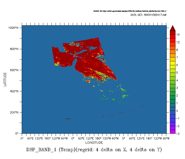
! We can see Florida and the Caribbean islands, but they are upside down.
! Ferret can use the netCDF library to address this, with the /ORDER qualifier.
yes? cancel data f99001082417.hdf
yes? use/ORDER=x-y "http://satdat1.gso.uri.edu:80/opendap/AVHRR/Old_Pathfinder/Northwest_Atlantic/6km/raw/1999/1/f99001082417.hdf"
! Note the odd axis labeling in the above plot. For these files, the coordinate axes are
! just index values, but the longitude/latitude ranges are defined in global attributes.
! We can redefine the x and y axes to represent the correct longitude and latitude axes.
yes? define axis/x=`..dsp_nav_earth_leflon`:`..dsp_nav_earth_ritlon`/npoints=1024/units=degrees_east `DSP_BAND_1,return=xaxis`
yes? define axis/y=`..dsp_nav_earth_botlat`:`..dsp_nav_earth_toplat`/npoints=1024/units=degrees_north `DSP_BAND_1,return=yaxis`
yes? shade/levels=v dsp_band_1[i=1:1024:4, j=1:1024:4]
yes? go land_detail