
Below is an annotated version of the script objective_analysis_demo.jnl
yes? go/help objective_analysis_demo.jnl

! Description: Demonstration of interpolating scattered data to grids
Two interpolation techniques are available for gridding.
Note that both of these are applicable ONLY for output grids which are REGULAR, that is to say, have EQUALLY-SPACEDcoordinates.
For simplicity this demo will work with abstract mathematicalfunctions rather than with "real" data. We will createan abstract function in the XY plane and use it as a model of"reality". Our goal is to sample this "reality"at scattered (X,Y) points and then attempt to recreate the originalfield through interpolation and objectibe analysis techniques.
Set up viewports and an abstract mathematical function to demonstrate the gridding technique.
DEFINE VIEW/ylim=.6,1/text=.5 vupperDEFINE VIEW/xlim=0.,.5/ylim=.3,.55/text=.2 vulDEFINE VIEW/xlim=.5,1./ylim=.3,.55/text=.2 vurDEFINE VIEW/xlim=0.,.5/ylim=0.05,.3/text=.2 vllDEFINE VIEW/xlim=.5,1./ylim=0.05,.3/text=.2 vlr
Define a 2-dimensional function and sample it
DEFINE AXIS/x=0:10:0.05 x10DEFINE AXIS/y=0:10:0.05 y10DEFINE GRID/x=x10/y=y10 g10x10SET GRID g10x10LET WAVE = SIN(KX*XPTS + KY*YPTS - PHASE) / 3LET PHASE = 0LET KAPPA = 0.4LET KX = 0.4LET KY = 0.7LET FCN1 = SIN(R)/(R+1)LET R = ((XPTS-X0)^2+ 5*(YPTS-Y0)^2)^0.5LET X0 = 3LET Y0 = 8LET sample_function = fcn1 + wave
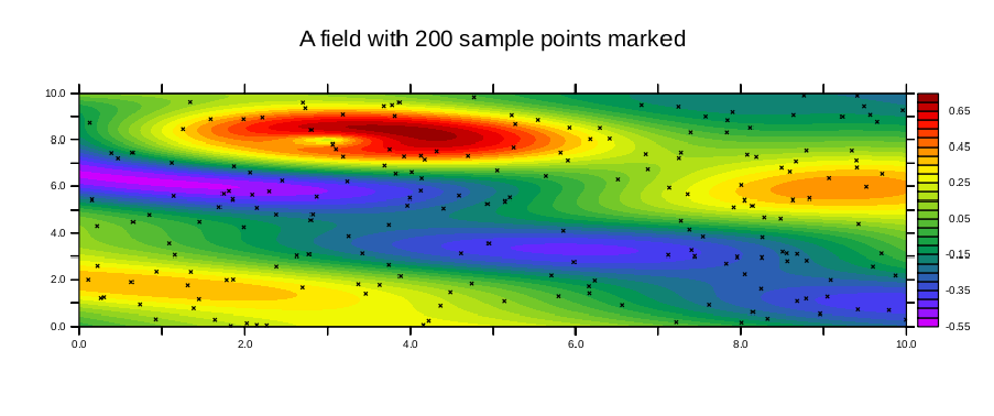
To display "reality" we will first let our sample points (xpts,ypts) be simply the X and y points of a grid. Then we will change (xpts,ypts) to be 200 sampling locations and mark them with symbols on the plot. We will draw this output in the "upper" viewport. The script draw_it simplifies plotting the functions in a viewport and with a title.
Shaded plot of the points on the (X,Y) grid
yes? set v upper
yes? fill/nolab  fcn1+wave
yes? annotate/norm/xpos=0.5/ypos=1.1/halign=0  "A field with 200 sample points marked"

! Store the color-levels to use for all the plots of gridded fields below.
yes? define symbol same_levels = /lev=(($lev_min),($lev_max),($lev_del))
Points randomly sampled in (X,Y), overlay the locations
yes? LET xpts = 10*randu(i); LET ypts = 10*randu(i+2)
yes? SET REGION/i=1:200
yes? PLOT/VS/OVER/SYMBOLS/NOLAB xpts,ypts
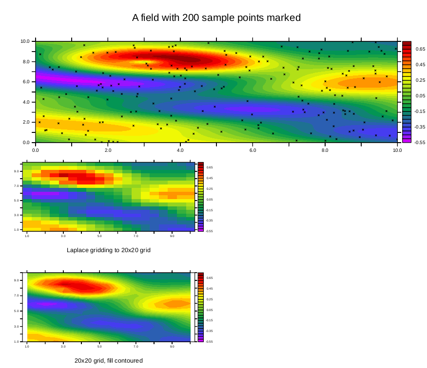
Now we will interpolate those 200 (X,Y,value) triples back onto a regular grid in the (X,Y) plane. The output grid will be from 1 to 10 by .5 along both the X and y axes. Defaults will be used for the interpolation controls. Under the "SHADEd" (raster-style) plot we will display the very same result as a filled contour.
yes? ! Define regularly-spaced output axes
yes?
yes? DEFINE AXIS/x=1:10:.5 xax5
yes? DEFINE AXIS/y=1:10:.5 yax5
yes? LET sgrid = scat2gridlaplace_xy (xpts, ypts, sample_function, x[gx=xax5], y[gy=yax5], 5., 5)
yes?
yes? set v vul
yes? shade($same_levels)/nolab sgrid
!-> shade/lev=(-0.55,0.75,0.05)/nolab sgrid
yes? annotate/norm/xpos=0.5/ypos=-0.3/halign=0 "Laplace gridding to 20x20 grid"

yes? set v vll
yes? fill($same_levels)/nolab sgrid
!-> CONTOUR/FILL/lev=(-0.55,0.75,0.05)/nolab sgrid
yes? annotate/norm/xpos=0.5/ypos=-0.3/halign=0 "20x20 grid, fill contoured"
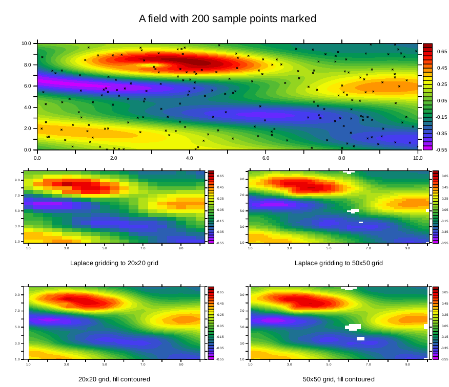
Now we perform the identical analysis but we will interpolate onto a higher resolution grid. The gaps in the output are because there are points on this output grid that are unacceptably far from any sample points using these interpolation parameters.
yes? DEFINE AXIS/x=1:10:.2 xax2
yes? DEFINE AXIS/y=1:10:.2 yax2
yes? LET sgrid = scat2gridlaplace_xy (xpts, ypts, sample_function, x[gx=xax2], y[gy=yax2], 5., 5)
yes?
yes? set v vur
yes? shade($same_levels)/nolab sgrid
!-> shade/lev=(-0.55,0.75,0.05)/nolab sgrid
yes? annotate/norm/xpos=0.5/ypos=-0.3/halign=0 "Laplace gridding to 50x50 grid"

yes? set v vlr
yes? fill($same_levels)/nolab sgrid
!-> CONTOUR/FILL/lev=(-0.55,0.75,0.05)/nolab sgrid
yes? annotate/norm/xpos=0.5/ypos=-0.3/halign=0 "50x50 grid, fill contoured"
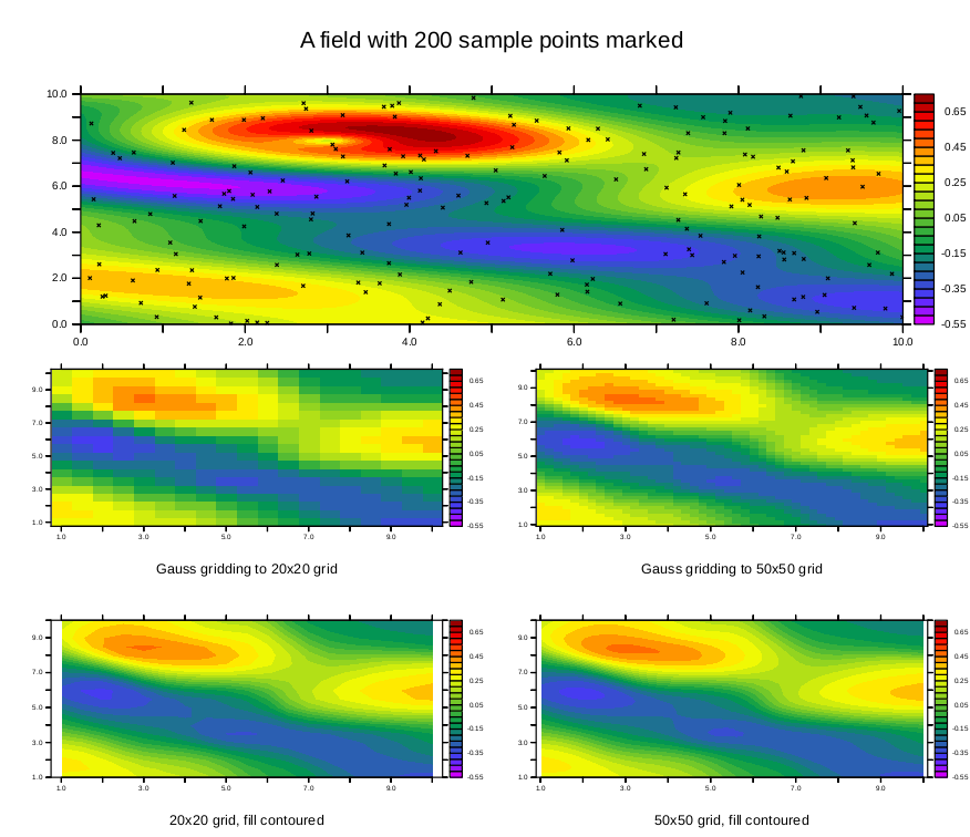
Now do the same plots with the Gaussian gridding function scat2gridgauss_xy which uses a different technique to interpolate the scattered points to the grid. This results in a somewhat smoother plot, however with these parameters, the result does not capture the extreme values. Using the same color scale on all plots makes this clear.. The interpolation parameters are XSCALE, YSCALE, XCUTOFF, YCUTOFF;where the algorithm uses scattered points which are within cutoff* the scale width from the gridbox center.
See also the FAQ, Calling SCAT2GRID functions for DSG data for some extra details when working with Discrete Sampling Geometries datasets.