
COADS is the comprehensive ocean-atmosphere data set compiled from ship reports over the global ocean. The monthly climatology introduced here represents a simple average of all data available for each month of the year from 1946-1989. The COADS dataset is a joint effort between NOAA's Physical Sciences Laboratory (Formerly the Climate Diagnostics Center (CDC)_ and the Cooperative Institute for Research in Environmental Sciences (CIRES) the National Center for Atmospheric Research (NCAR), and NOAA's National Centers for Environmental Information(NCEI)
Use of FERRET commands in the tour will give you a good idea how useful the program can be exploring data sets. Commands to FERRET below will be in capital letters. FERRET prompts for input with the word "yes?".
yes? SET DATA coads-climatology
yes? SHOW DATA coads-climatology

currently SET data sets:
1> ./coads-climatology.des (default)
name title I J K L
SST SEA SURFACE TEMPERATURE 1:180 1:90 1:1 1:12
AIRT AIR TEMPERATURE 1:180 1:90 1:1 1:12
SPEH SPECIFIC HUMIDITY 1:180 1:90 1:1 1:12
WSPD WIND SPEED 1:180 1:90 1:1 1:12
UWND ZONAL WIND 1:180 1:90 1:1 1:12
VWND MERIDIONAL WIND 1:180 1:90 1:1 1:12
SLP SEA LEVEL PRESSURE 1:180 1:90 1:1 1:12
Note that 7 variables are available. The grid is 2x2 degree, and global. For information on FERRET's grid indices click here.
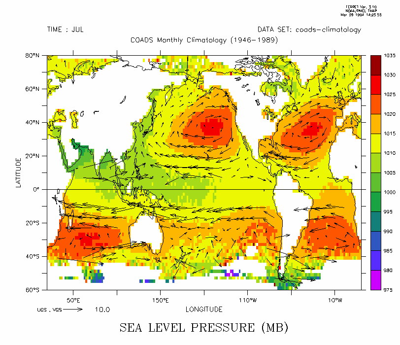
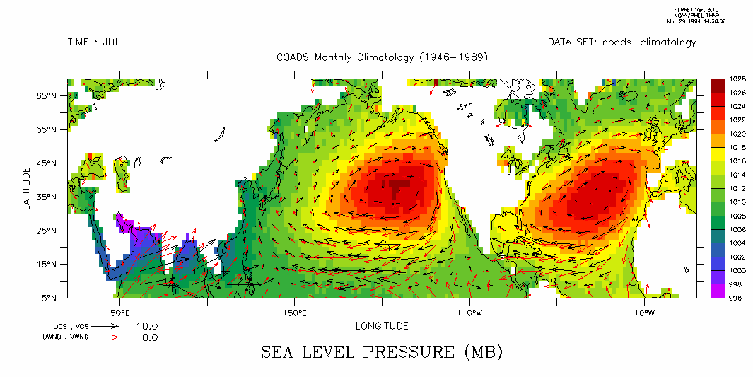
The following commands will generate a plot of sea level pressure and winds for the average July.
yes? SET REGION/Y=60S:80N
yes? SHADE/L=7 SLP
yes? GO land
yes? VECTOR/OVER/L=7/LEN=10 UWND,VWND

The horizontal equations of motion on the rotating earth show that acceleration of a parcel of air is dependent on the pressure gradient, the Coriolis force, and any friction retarding its motion. Neglecting friction, a geostrophic wind may be defined, where the pressure gradient force is balanced by the Coriolis force. Let's define variables ug and vg to be that geostrophic wind, being careful to use common units of measure.
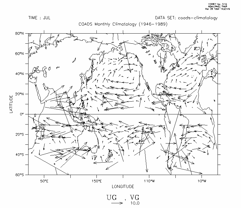
The commands below produce a plot of the geostrophic wind. The geostrophic wind is ill-defined near the equator, as f is 0 there. This definition specifies ug and vg poleward of latitudes +/- 5 degrees.
yes? LET RHO = 1.275 Use a constant for air density for now
yes? LET OMEGA = 2*3.14159/86400 The angular velocity of the earth
yes? LET DPDX = SLP[X=@DDC]*100 Zonal pressure gradient (in SI units)
yes? LET DPDY = SLP[Y=@DDC]*100 Meridional pressure gradient
yes? LET C = 3.14159/180 Conversion factor -- radians/degree
yes? LET F = 2*OMEGA*SIN(Y[G=COADS1]*C) The coriolis parameter

yes? LET/TITLE="VG" VG = IF ABS(Y) GT 5 THEN DPDX/(F*RHO)
yes? LET/TITLE="UG" UG = IF ABS(Y) GT 5 THEN (-1)*DPDY/(F*RHO)

yes? VECTOR/LEN=10/L=7 UG,VG
yes? GO land
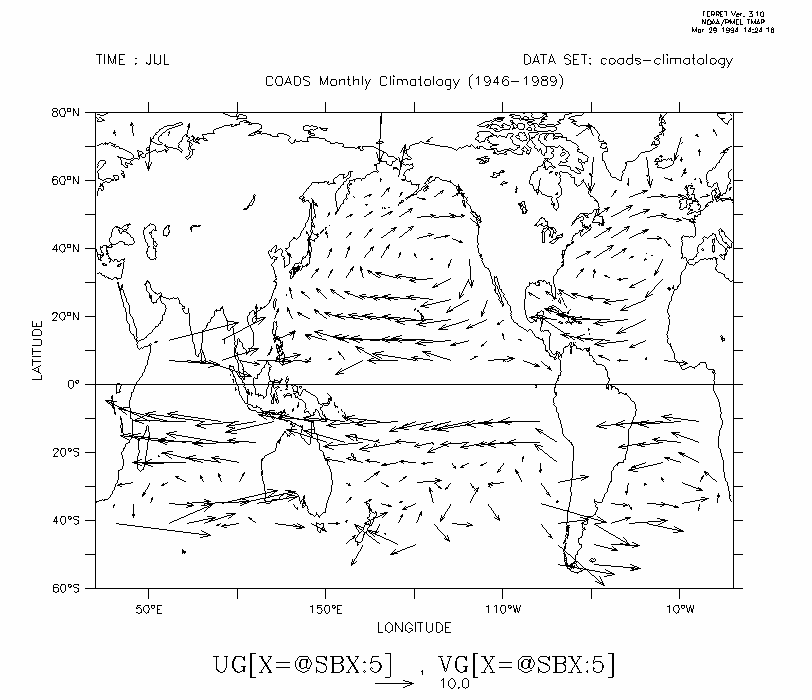
A bit noisy so let's smooth it 5 grid points in x:
yes? LET UGS = UG[X=@SBX:5]
yes? LET VGS = VG[X=@SBX:5]
yes? VECTOR/LEN=10/L=7 UGS,VGS
yes? GO land
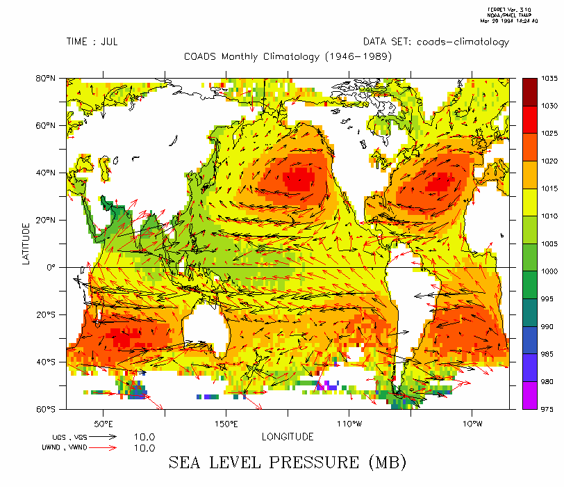
Here is the geostrophic wind field superimposed on sea level pressure:
yes? SHADE/L=7 SLP
yes? GO land
yes? VECTOR/LEN=10/OVER/L=7 UGS,VGS
overlay the observed winds we see that they are often subgeostrophic, that is, the Coriolis force is not strong enough to balance the pressure gradient force (from high to low pressure), possibly indicating presence of friction near the earth's surface:
yes? VECTOR/LEN=10/OVER/L=7 UWND,VWND
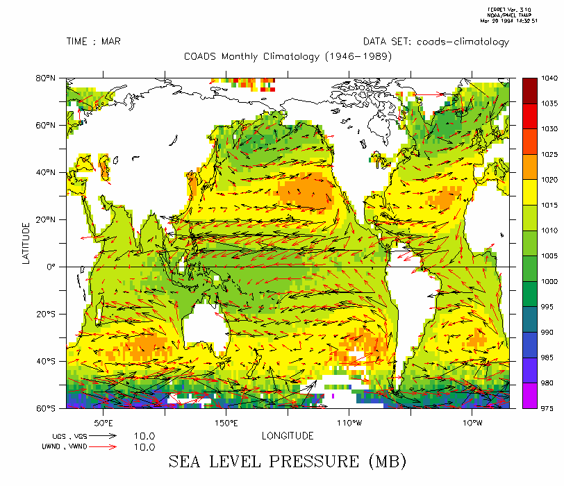
Here's the same plot for March:
yes? SHADE/L=3 SLP
yes? GO land
yes? VECTOR/LEN=10/OVER/L=3 UGS,VGS
yes? VECTOR/LEN=10/OVER/L=3 UWND,VWND
And we can look more closely at a hemisphere:
SET REGION/Y=5:70
SET WIND/ASP=.5

SHADE/L=7 SLP
GO land
VECTOR/LEN=10/OVER/L=7 UGS,VGS
VECTOR/LEN=10/OVER/L=7 UWND,VWND
Much more exploration of the global climate is possible using the COADS climatology. This tour uses a fixed value for the density of air. Since pressure, temperature, and specific humidity are available, density could be cast in a more complex functional form. Models of the friction suggested above can be tested -- and other explorations that come to mind.