Below is an annotated version of the script ef_eof_demo.jnl
Demonstration of computing EOFs using the External Functions EOFSVD_SPACE, EOFSVD_TFUNC, EOFSVD_STAT
Please see the Ferret documentation for full details and references to the source of these functions.
-
EOFSVD_SPACE returns EOF eigenvectors: spatial EOF in x and y with the same units as the incoming data
-
EOFSVD_TFUNC returns EOF time amplitude functions; dimensionless
-
EOFSVD_STAT returns statistics on the EOF computation: number of EOFs scaled and returned; Percent variance explained by each EOF; and the eigenvalues.
Example 1: Define a function of x,y,time using trig functions. Decompose into spatial and time EOF's and display statistics.
yes? LET time = t[t=1-jan-1990:10-jan-1990:24]   ! 24 hour resolution time axis

yes? DEFINE AXIS/x=0:10:0.5 x10
yes? DEFINE AXIS/y=0:10:0.5 y10
yes? DEFINE GRID/x=x10/y=y10/t=time g10x10
yes? SET GRID g10x10

yes? LET fcn1 = 15.* sin(omega1*t)*cos(r)/(r+1)
yes? LET fcn2 = 20.* sin(omega2*t)*(sin(s)-.2*sin(q))/(s+1)

yes? LET r = ((6.*(xpts-x0)^2 + 7.*(ypts-y0)^2)^0.5)
yes? LET s = (((xpts-x1)^2 + 2*(ypts-y1)^2)^0.5)
yes? LET q = ((3*(xpts-x0)^2 + (ypts-y1)^2)^0.5)

yes? LET x0 = 2
yes? LET y0 = 4
yes? LET x1 = 5
yes? LET y1 = 7

yes? LET omega1 = 1/10*2*3.14159
yes? LET omega2 = 2 * omega1

yes? LET sample_function = fcn1 + fcn2
yes? LET xpts = x
yes? LET ypts = y
Compute the statistics on the EOF solution. EOF_STAT returns:
- for J=1 the number of EOFs returned
- for J=2 the percent variance explained by each EOF
- for J=3 the eigenvalue for each EOF
yes? LET estat = EOFSVD_STAT(sample_function)

yes? LIST/I=1/J=1 estat
EOFSVD_STAT(SAMPLE_FUNCTION)
X: 1
Y: 1
2.000

yes? LIST/I=1:4/J=2 estat
EOFSVD_STAT(SAMPLE_FUNCTION)
2
1   / 1:  93.59
2   / 2:   6.41
3   / 3:   0.00
4   / 4:   0.00

yes? LIST/I=1:4/J=3 estat
EOFSVD_STAT(SAMPLE_FUNCTION)
3
1   / 1:  1104.
2   / 2:    76.
3   / 3:     0.
4   / 4:     0.
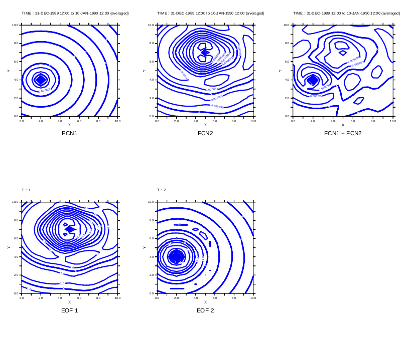
Plot the original function (averaged over time) and its spatial decomposition by EOFSVD_SPACE
Define some viewports...
yes? DEFINE VIEW/xlim=0.,.33/ylim=.6,1./text=0.2 vul
yes? DEFINE VIEW/xlim=.33,.66/ylim=.6,1./text=0.2 vuc
yes? DEFINE VIEW/xlim=.66,1./ylim=.6,1./text=0.2 vur

yes? DEFINE VIEW/xlim=0.,.33/ylim=.1,.5/text=0.2 vll
yes? DEFINE VIEW/xlim=.33,.66/ylim=.1,.5/text=0.2 vlc
yes? DEFINE VIEW/xlim=.66,1./ylim=.1,.5/text=0.2 vlr
Plot the functions we used to synthesize the example function
yes? SET VIEW vul; CONTOUR/TITLE="FCN1" fcn1[l=1:10@ave]
yes? SET VIEW vuc; CONTOUR/TITLE="FCN2" fcn2[l=1:10@ave]
yes? SET VIEW vur; CONTOUR/TITLE="FCN1 + FCN2" sample_function[l=1:10@ave]
Plot the decomposition by EOFSVD_SPACE
yes? LET exy = EOFSVD_SPACE(sample_function, 0.1)

yes? SET VIEW vll; CONTOUR/L=1/TITLE="EOF 1" exy
yes? SET VIEW vlc; CONTOUR/L=2/TITLE="EOF 2" exy
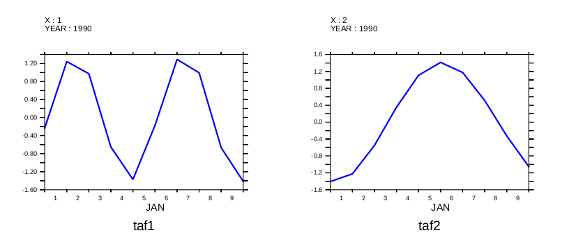
Now compute and plot the time amplitude functions.
yes? LET etim = EOFSVD_TFUNC(sample_function)


yes? SET VIEW ul
yes? plot/color=blue/thick/I=1/TITLE=taf1 etim

yes? SET VIEW ur
yes? plot/color=blue/thick/I=2/TITLE=taf2 etim
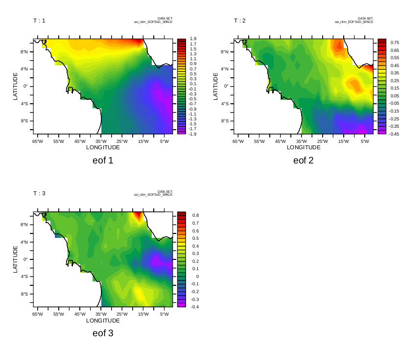
Example 2: Using the COADS climatology data.
yes? USE coads_climatology

!  Compute and save the spatial EOF functions.  These have the same units
!  as the data.

yes? LET EOF_xyfcn = EOFSVD_SPACE(sst[X=67w:1w,Y=11S:11N])
yes? SAVE/CLOBBER/FILE=sst_clim_EOFSVD_SPACE.cdf eof_xyfcn

yes? CANCEL DATA/ALL
yes? CANCEL VARIABLE/ALL
yes? CANCEL REGION
Plot the first three eigenfunctions
yes? USE sst_clim_EOFSVD_SPACE.cdf

yes? SET VIEW ul; fill/l=1/TITLE="eof 1" eof_xyfcn; go land
yes? SET VIEW ur; fill/l=2/TITLE="eof 2" eof_xyfcn; go land
yes? SET VIEW ll; fill/l=3/TITLE="eof 3" eof_xyfcn; go land
Compute the statistics on the EOFs: number of EOFs scaled and returned; Percent variance explained by each EOF; and the eigenvalues.
yes? USE coads_climatology
yes? LET eofstat = EOFSVD_STAT(sst[X=67w:1w,Y=11S:11N])

yes? let nout = eofstat[i=1,j=1]
yes? let pcts = eofstat[i=1:`nout`,j=2]
yes? let eigenv = eofstat[i=1:`nout`,j=3]

yes? LIST nout
VARIABLE : EOFSTAT[I=1,J=1]
FILENAME : coads_climatology.cdf
FILEPATH : /home/users/tmap/ferret/linux/fer_dsets/data/
X        : 1
Y        : 1
284.0


yes? LIST/I=1:6 pcts
VARIABLE : EOFSTAT[I=1:284,J=2]
FILENAME : coads_climatology.cdf
FILEPATH : /home/users/tmap/ferret/linux/fer_dsets/data/
SUBSET   : 6 points (X)
Y        : 2
2
2
1   / 1:  86.95
2   / 2:   5.82
3   / 3:   3.87
4   / 4:   1.51
5   / 5:   0.56
6   / 6:   0.38

yes? LIST/I=1:6 eigenv
VARIABLE : EOFSTAT[I=1:284,J=3]
FILENAME : coads_climatology.cdf
FILEPATH : /home/users/tmap/ferret/linux/fer_dsets/data/
SUBSET   : 6 points (X)
Y        : 3
3
3
1   / 1:  249.4
2   / 2:   16.7
3   / 3:   11.1
4   / 4:    4.3
5   / 5:    1.6
6   / 6:    1.1
Compute and plot time amplitude functions: Note they are dimensionless.
yes? USE coads_climatology
yes? LET eoftime = EOFSVD_TFUNC(sst[X=67w:1w,Y=11S:11N])

SAVE/CLOBBER/FILE=sst_clim_eof_tfunc.cdf eoftime[i=1:`nout`]

yes? CANCEL VARIABLE/ALL
yes? CANCEL VIEW
yes? USE sst_clim_eof_tfunc.cdf

yes? SET VIEW ul
yes? plot/color=blue/thick/I=1/TITLE="time function 1"/VLIMITS=-2:2:0.5 eoftime
yes? SET VIEW ur
yes? plot/color=blue/thick/I=2/TITLE="time function 2"/VLIMITS=-2:2:0.5 eoftime
yes? SET VIEW ll
yes? plot/color=blue/thick/I=3/TITLE="time function 3"/VLIMITS=-2:2:0.5 eoftime
